Tutorial 3

Author

Affiliation

Matéo Moglia

CREST - Institut Polytechnique de Paris

Published

May 5, 2025

Roadmap

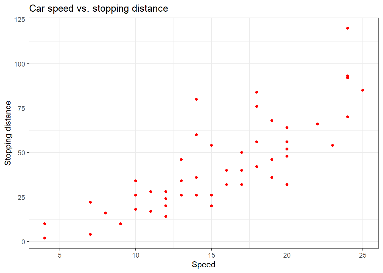
For this third tutorial, we are going to

Recap on the OLS estimation
Learn how to go from a model to an empirical prediction
Replicate the key results from Mankiw, Romer, Weil (1994)

Note

Big disclaimer: the recap on OLS is hugely inspired from Florian Oswald’s and Sciences Po’s introduction to Econometrics with R. The interested student can check this fantastical material here: scpoecon.github.io.

Linear regression

Why? When?

An empirical tool to assess the statistical relationship between variables
In the toolbox of the social scientist, with many other tools
Correlation is not causation

Topic of today: Ordinary Least Square estimator (which is a widely used estimator)

Tip

Keep in mind the difference between an estimator \(\hat \beta\) and the observed value \(\beta\). We cannot observe the true parameter, so we estimate it (with error).

Linear regression

Visual intuition

We use the cars dataset, in base R, and we are going to relate how speed and stopping distance are related.

ggplot(cars,aes(x=speed,y=dist)) +
  geom_point(color="red") +
  xlab("Speed") + ylab("Stopping distance") +
  ggtitle("Car speed vs. stopping distance") +
  theme_bw()

Linear regression

Visual intuition

It seems that a line could be helpful to “summarize” the relation between both variables!

ggplot(cars,aes(x=speed,y=dist)) +
  geom_point(color="red") +
  geom_abline(intercept=10,slope=2.5,color="blue") +
  xlab("Speed") + ylab("Stopping distance") +
  ggtitle("Car speed vs. stopping distance") +
  theme_bw()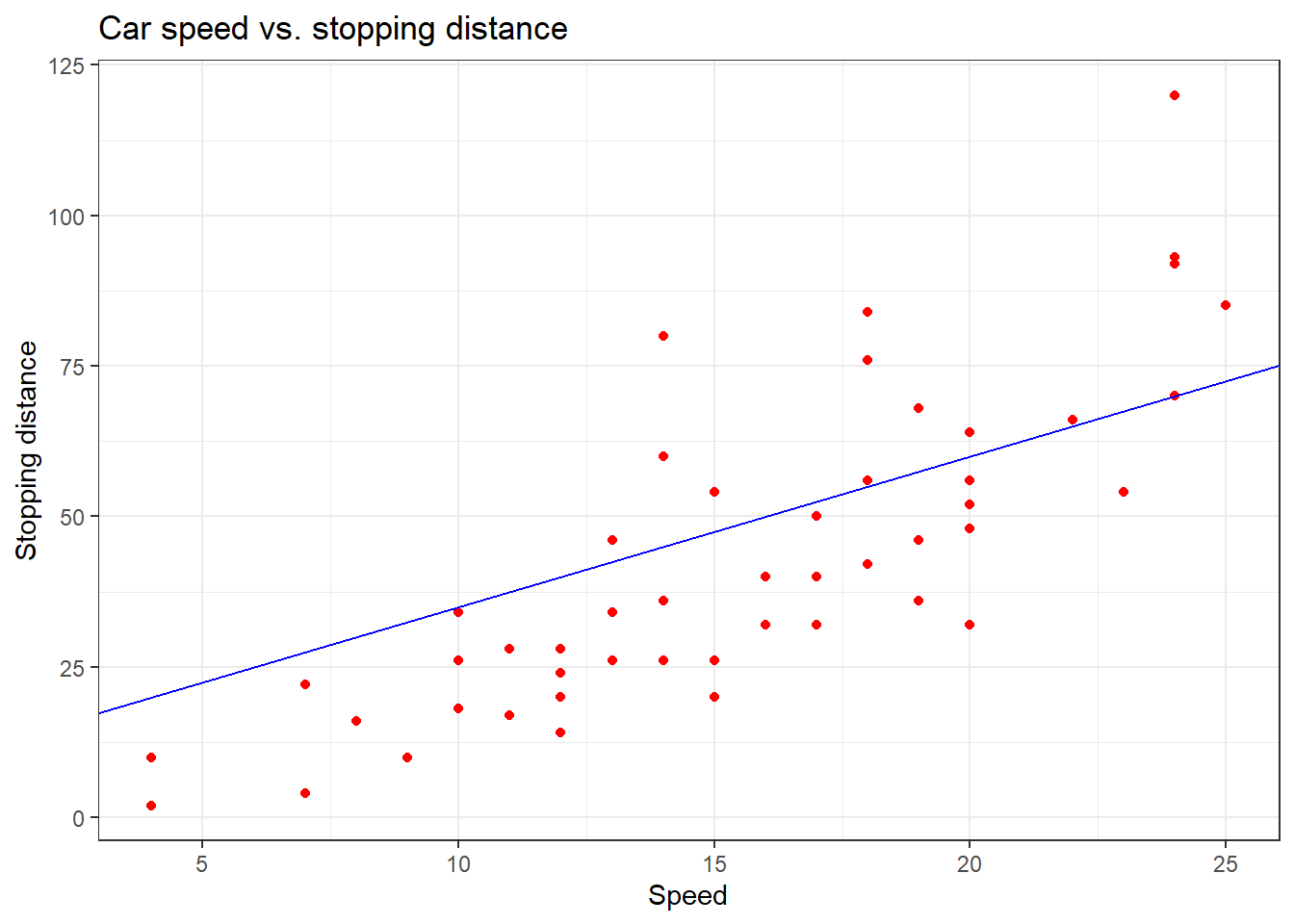

Linear regression

Bringing some maths

We want to minimize the distance between the line and the points
In practice, the sum of distances can go to 0. Solution?

ggplot(cars, aes(x = speed, y = dist)) +
  geom_point(color = "black") +
  geom_abline(intercept = 5, slope = 2.5, color = "blue") +
  geom_segment(aes(x = speed, 
                   y = dist, 
                   xend = speed, 
                   yend = 5 + 2.5 * speed), 
               arrow = arrow(length = unit(0.1, "inches")), 
               color = "red") +
  xlab("Speed") + 
  ylab("Stopping distance") +
  ggtitle("Car speed vs. stopping distance") +
  theme_bw()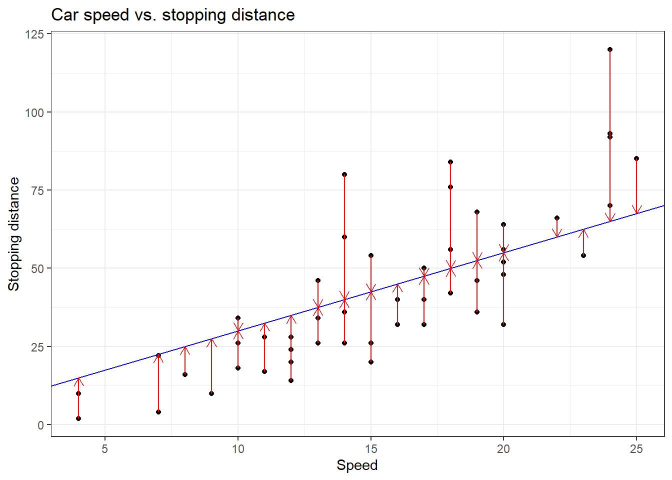

Linear regression

Bringing some maths

We compute the sum of square distances (\(\sim\) error), so the name “ordinary least square”
An affine function is defined as \(y = \beta_0 + \beta_1 x\) which in matrix form gives \(Y = X\beta\).
Dimension of \(X\)?
The error for each observation is \(e_i = y_i - \beta_0 - \beta_1 x_i\)
Hence, we look for \(\beta\) such that: \[ \beta^\star = \min_\beta (Y - X\beta)'(Y - X\beta) = \min_\beta e'e \]
First order condition: derivative wrt \(\beta\) should be equal to 0

Linear regression

Defining the OLS estimator

The OLS estimator is then: \[ \hat{\beta} = (X'X)^{-1}X'y \]
Who wants to try to derive it?
Under some conditions, this estimator is the Best Linear Unbiased Estimator (BLUE)
Those conditions will be super helpful later

Linear regression

Gauss-Markov theorem

Linearity
- The relationship has to be linear
- See Anscombe quartet
- Solutions: \(\log\), squared
\(X\) is full rank
- Ensure that variables are not perfectly colinear
- There are more observations than variables (\(n > k\))
Zero conditional mean
- Errors are not correlated with \(X\) (exogeneity)
Homoskedasticity
- Errors are not correlated between observations
- Solutions: robust estimation

Linear regression

Gauss-Markov theorem violation

Major threat is 3 (= endogeneity). Usually it arises from 2 sources:

Reverse causality. Any exemple?
Omitted Variable Bias. Any exemple?

Then, the OLS estimator is biased and \(E(\widehat\beta)\neq \beta\). Proof in appendix.

It also means that \(Cov(Y,\epsilon)\neq 0\). In other words, that \(y\) and \(\epsilon\) somehow move jointly due to some unobserved factors and not due only to variation due to \(X\).

We will see many ways to tackle this issue.

Today: Omitted Variable Bias
Next week: Endogeneity.

Tip

Extensive presentation of the derivations and the Gauss-Markov theorem here.

A third case leads to an unbiased estimator with higher standard errors (not the best estimator anymore): measurement error. The intuition behind measurement error is more straightforward:

If \(x = x^\star + \delta\) where \(\delta\) is a measurement error with mean 0, then the estimator is still unbiased but the variance is higher and the estimation is leess precise.

Linear regression

R2 and prediction quality

R2 is the coefficient of determination, assessing the share of total variance explained by the model

\[\small R^2 = \frac{\texttt{Variance explained}}{\texttt{Total variance}} = \frac{\text{Sum of explained square}}{\text{Total sum of square}} = 1 - \frac{\text{Sum of square residuals}}{\text{Total sum of square}} \]

R2 is between 0 and 1
The higher the R2, the larger the share of variance explained by the model
A low R2 is not necessarily bad: it is just that the model explains a low share of variance

Linear regression

Interpretation

Once the model set, we can estimate it using R functions
Main function is lm. For linear model, the syntax is lm(y ~ x)

summary(lm(cars$dist ~ cars$speed))


Call:
lm(formula = cars$dist ~ cars$speed)

Residuals:
    Min      1Q  Median      3Q     Max 
-29.069  -9.525  -2.272   9.215  43.201 

Coefficients:
            Estimate Std. Error t value Pr(>|t|)    
(Intercept) -17.5791     6.7584  -2.601   0.0123 *  
cars$speed    3.9324     0.4155   9.464 1.49e-12 ***
---
Signif. codes:  0 '***' 0.001 '**' 0.01 '*' 0.05 '.' 0.1 ' ' 1

Residual standard error: 15.38 on 48 degrees of freedom
Multiple R-squared:  0.6511,    Adjusted R-squared:  0.6438 
F-statistic: 89.57 on 1 and 48 DF,  p-value: 1.49e-12

Results are significant (low p-value), R2 is relatively large

Linear regression

P-value

The Pr(>|t|) value is also called the p-value. Let’s assume that we want to have a significance level \(\alpha\) of 5%. The underlying statistical test is the following:

\[ \begin{align*} H_0 : \beta = 0 \\ H_1 : \beta \neq 0 \end{align*} \]

where \(\beta\) is the true coefficient.

We want to know if, conditional on the fact that \(H_0\) is true (the true parameter value is 0), \(\widehat \beta = 3.93\) is due to pure chance (then we keep \(H_0\)) or if it cannot be due to chance (and we reject \(H_0\)).

If the p-value falls below the threshold \(\alpha\), then we can confidently assume that the coefficient is significantly different from 0. In other words, we reject the hypothesis that the speed has no influence on the stopping distance at the 5% level.

For more details, you can check this quick note.

Linear regression

Interpretation

Note

Everything should be intepreted everything else equal!

Level-level regression: marginal effect. If \(x\) increases by 1, \(y\) increases by \(\beta\)
Log-log regression: elasticity. If \(x\) increases by 1%, \(y\) increases by \(\beta\)%
Log-level regression: percentage change. If \(x\) increases by 1, \(y\) increases by \(100\beta\)
Level-log regression: level change. If \(x\) increases by 1%, \(y\) increases by \(\beta/100\)

From the model to the data

Solow model

Using Harrod-neutral technological progress, the GDP per capita equation is: \[\small \frac{Y(t)}{L(t)} = K(t)^\alpha (A(t) L(t))^{1-\alpha} \quad \alpha \in \ (0,1) \]
We assume an exogenous growth rate of \(A\) and \(L\) such that: \(A(t) = A(0)e^{gt}\) and \(L(t) = L(0) e^{nt}\).
At the steady-state level:

\[\small \frac{Y}{L} = A(0)e^{gt}\left(\frac{s}{n + g + \delta}\right)^{\alpha/(1-\alpha)} \]

Super convenient: we can measure everything
- \(Y/L\), GDP divided by working age population
- \(s\), saving measured as the real investment
- \(n\), population growth rate
- \(\delta\) and \(g\), capital depreciation and growth rate of technology (assumed constant)

From the model to the data

Is this relationship linear?

No. Solution?

Log-linearize it (at time 0)

\[ \log (Y/L) = \log(A(0)) + \left(\frac{\alpha}{1-\alpha}\right)\log s - \left(\frac{\alpha}{1-\alpha}\right) \log(n + g + \delta) \]

From the model to the data

Empirical model

Because we do not observe all data, we can only estimate the parameters. Hence, the empirical model we estimate is:

\[ \log (Y_i/L_i) = \beta_0 + \beta_1 \log s_i + \beta_2 \log(n + g + \delta) + \epsilon_i \]

where \(\beta_0 + \epsilon_i = \log A(0)\), and \(\epsilon_i\) is an error term capturing everything not captured in the model.

Note

We can, or not, assume that \(\beta_1 = -\beta_2\). This is an empirical prediction we might want to test.

Exercise

Data cleaning and descriptive statistics

Load the data and the packages (dplyr and ggplot2)
What are the three groups of countries in the data?
Compute summary statistics based on country group
Plot the growth rate of GDP per capita vs. the log of GDP per capita

Exercise

Baseline estimation

Assume \(g+\delta=0.05\).

Generate the variables you need in the regression
Run the model on the full sample and on each sub-group. Store the results in appropriate objects.
- [Bonus] Use a loop to do it
Interpret the results in the light of the Solow model predictions. What is the share of cross-country income per capita variation is explained by the model?
[Bonus] We assumed that \(\beta_1 \neq -\beta_2\). Using linearHypothesis() from the package car, you can set an hypothesis testing to check if the sum of the coefficient is equal to 0.
In previous work, the share of capital in production was thought to be roughly 1/3, is this prediction supported by the data?

Exercise

Adding the human capital

Does the previous model violate the exogeneity assumption? Why?
A proposed solution is to add a new variable to capture the level of human capital: school.
Run again the model on the full and sub- samples.
Interpret.
Export the tables and the graph in LaTeX

Appendix

Anscombe quartet

g1 = ggplot(datasets::anscombe,aes(x=x1,y=y1)) +
  geom_point(color="black") +
  geom_smooth(method = "lm",se=F) +
  theme_bw() +
  xlab("X") + ylab("Y") + ggtitle("Q1")
g2 = ggplot(datasets::anscombe,aes(x=x2,y=y2)) +
  geom_point(color="black") +
  geom_smooth(method = "lm",se=F) +
  theme_bw() +
  xlab("X") + ylab("Y") + ggtitle("Q2")
g3 = ggplot(datasets::anscombe,aes(x=x3,y=y3)) +
  geom_point(color="black") +
  geom_smooth(method = "lm",se=F) +
  theme_bw() +
  xlab("X") + ylab("Y") + ggtitle("Q3")
g4 = ggplot(datasets::anscombe,aes(x=x4,y=y4)) +
  geom_point(color="black") +
  geom_smooth(method = "lm",se=F) +
  theme_bw() +
  xlab("X") + ylab("Y") + ggtitle("Q4")

(g1 | g2) /
(g3 | g4)

`geom_smooth()` using formula = 'y ~ x'
`geom_smooth()` using formula = 'y ~ x'
`geom_smooth()` using formula = 'y ~ x'
`geom_smooth()` using formula = 'y ~ x'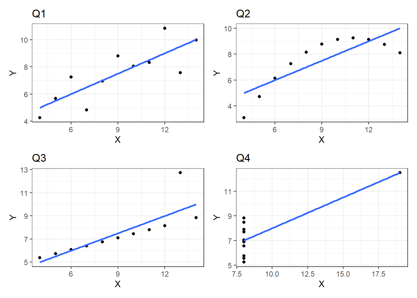

Appendix

Omitted variable bias proof

Omitted Variable Bias (OVB) occurs when a relevant variable is left out of a regression model, leading to biased and inconsistent estimators. Here, we formally prove the presence of bias in the Ordinary Least Squares (OLS) estimator due to an omitted variable.

Consider the true model: \(Y = \beta_0 + \beta_1 X_1 + \beta_2 X_2 + \epsilon\) where \(Y\) is the dependent variable, \(X_1\) and \(X_2\) are explanatory variables, \(\epsilon\) is the error term with \(E[\epsilon | X_1, X_2] = 0\).

Now, suppose \(X_2\) is omitted from the regression. The estimated model is: \[ Y = \alpha_0 + \alpha_1 X_1 + u \]

where the new error term \(u\) is: \(u = \beta_2 X_2 + \epsilon\). Since \(X_2\) is omitted, we express it in terms of \(X_1\) using the linear projection:

\[ X_2 = \gamma_0 + \gamma_1 X_1 + v \]

where \(v\) is the residual such that \(E[v | X_1] = 0\).

Substituting this into the omitted equation:

\[ u = \beta_2 (\gamma_0 + \gamma_1 X_1 + v) + \epsilon \]

\[ u = \beta_2 \gamma_0 + \beta_2 \gamma_1 X_1 + \beta_2 v + \epsilon \]

Since \(u\) is correlated with \(X_1\), the OLS estimator for \(\alpha_1\) (which is another way to write an estimator) is:

\[ \hat{\alpha}_1 = \frac{Cov(Y, X_1)}{Var(X_1)} \]

Substituting \(Y\) from the true model:

\[ \hat{\alpha}_1 = \frac{Cov(\beta_0 + \beta_1 X_1 + \beta_2 X_2 + \epsilon, X_1)}{Var(X_1)} \]

Expanding covariance terms:

\[ \hat{\alpha}_1 = \beta_1 + \beta_2 \frac{Cov(X_2, X_1)}{Var(X_1)} \]

Using the projection equation:

\[ \hat{\alpha}_1 = \beta_1 + \beta_2 \gamma_1 \]

Since \(\gamma_1 \neq 0\) if \(X_1\) and \(X_2\) are correlated, and \(\beta_2 \neq 0\) if \(X_2\) is relevant, it follows that:

\[ E[\hat{\alpha}_1] \neq \beta_1 \]

Thus, the OLS estimator is biased due to the omission of \(X_2\). Another way of seeing it on these slides.

Other Formats

Roadmap

Linear regression

Why? When?

Linear regression

Visual intuition

Linear regression

Visual intuition

Linear regression

Bringing some maths

Linear regression

Bringing some maths

Linear regression

Defining the OLS estimator

Linear regression

Gauss-Markov theorem

Linear regression

Gauss-Markov theorem violation

Linear regression

R2 and prediction quality

Linear regression

Interpretation

Linear regression

P-value

Linear regression

Interpretation

From the model to the data

Solow model

From the model to the data

Is this relationship linear?

From the model to the data

Empirical model

Exercise

Data cleaning and descriptive statistics

Exercise

Baseline estimation

Exercise

Adding the human capital

Appendix

Anscombe quartet

Appendix

Omitted variable bias proof